

For most FX portfolios, the right answer is not one model but a hierarchy: variance-covariance for fast daily monitoring, historical simulation as the workhorse for board reporting, and Monte Carlo when options or other non-linear positions enter the book. None of that matters if the holding period does not match the actual hedge cycle or if backtesting against FCA BIPRU7 standards gets skipped. CorpHedge treats those two disciplines, horizon alignment and rigorous validation, as the floor for any FX VaR model, at 95% or 99% confidence.
TL;DR:
- Using historical simulation for VaR provides the most realistic assessment of fat tails and skew, but relies heavily on the relevancy of the historical window.
- Monte Carlo simulation is necessary when options or non-linear FX instruments are involved, despite higher computational costs and model risks.
- Volatility inputs should be backtested and chosen through stress tests between EWMA and GARCH models, rather than relying on simple square-root-of-time scaling.
- Data quality, including appropriate window length, cleaning, and correlation stability, is critical to producing reliable VaR estimates, especially during regime changes.
- Combining VaR with a governance process that includes regular backtesting, stress testing, and model validation ensures meaningful risk controls and regulatory compliance.
Table of Contents
- Core FX VaR Methods: Variance-Covariance, Historical Simulation, and Monte Carlo
- Choosing Volatility Inputs, Weighting, and Horizon Scaling
- Data Quality: Windows, Cleaning, and Correlation Stability
- Backtesting: Hit Rates, Exceptions, and Regulatory Expectations
- Turning VaR Into Treasury Limits and Hedging Decisions
- Advanced Extensions: EVT, CAViaR, and Machine Learning Approaches
- How CorpHedge Supports the FX VaR Workflow
- FX VaR Compared to CVaR and Expected Shortfall
- Liquidity, Market Microstructure, and What They Do to VaR
- Implementation Challenges and the Software Layer
- Regulatory Requirements and Compliance Considerations
- Case Studies: VaR Under Different Market Conditions
- The Governance-First View on FX VaR
- CorpHedge: Turning FX VaR Into a Daily Workflow
- Sources
- FAQ
Core FX VaR Methods: Variance-Covariance, Historical Simulation, and Monte Carlo
Three methods dominate FX VaR modeling: variance-covariance (parametric), historical simulation, and Monte Carlo simulation. Each rests on a different assumption about how currency returns behave, and that assumption determines where the method breaks.
Parametric VaR assumes returns follow a normal (or sometimes Student's t) distribution and calculates risk from a covariance matrix of currency pairs. It is fast, computationally cheap, and easy to explain to a treasury committee that does not want a statistics lecture. The catch: FX returns exhibit fat tails and volatility clustering, so parametric VaR routinely understates the risk of extreme moves, particularly around central bank surprises or liquidity shocks.
Historical simulation avoids the distributional assumption entirely. It reprices the current portfolio using actual historical return paths, typically 250 to 500 days, then reads the VaR off the resulting loss distribution. This handles fat tails and skew naturally, but it is only as good as the window you feed it. A 2020 crisis window baked into your 2026 dataset will inflate VaR long after the shock has passed, unless you weight it deliberately.
Monte Carlo simulation generates thousands of hypothetical return paths from a specified stochastic process, then values the portfolio under each. It is the only practical choice once options, barriers, or other non-linear FX instruments enter the picture, since neither parametric nor historical methods handle convexity well. The tradeoff is compute cost and model risk: the output is only as trustworthy as the volatility and correlation assumptions driving the simulation. The RBA's research on VaR and backtesting techniques walks through the calculation mechanics of all three approaches and how they perform against realized losses.
Picking a starting method comes down to three questions:
- Portfolio complexity. A linear forward book fits parametric or historical simulation; anything with optionality needs Monte Carlo.
- Instrument non-linearity. If delta alone does not describe your exposure, skip parametric VaR.
- Data availability. Thin history on an exotic pair pushes you toward parametric methods with proxy inputs, not historical simulation.
Most treasury teams end up running historical simulation as the primary number and parametric VaR as a same-day sanity check.
Choosing Volatility Inputs, Weighting, and Horizon Scaling
Volatility modeling is where FX VaR models actually go wrong, more often than method selection. Two competing approaches dominate: exponentially weighted moving average (EWMA) and GARCH.
EWMA weights recent observations more heavily using a single decay parameter, usually between 0.94 and 0.97 for daily FX data. It reacts quickly to regime shifts, which matters when a currency pair suddenly starts trading like a different instrument after a rate decision. GARCH models volatility as a function of past shocks and past variance, capturing mean reversion in volatility that EWMA misses. GARCH tends to outperform in stable regimes; EWMA tends to react faster in turning markets. Neither is categorically better, which is why serious desks run both and compare.
Here is a practical sequence for setting up the volatility engine:
- Pull at least two years of daily FX returns for every pair in the exposure.
- Fit both EWMA (test decay factors between 0.94 and 0.99) and a GARCH(1,1) baseline.
- Backtest each against realized volatility over rolling 20-day windows.
- Stress-test parameter sensitivity by shifting the decay factor by ±0.02 and checking how much VaR moves.
- Lock the choice into a model-change log before production use.
The most common scaling error in corporate FX risk management is naive square-root-of-time extrapolation, taking a 1-day VaR and multiplying by the square root of the holding period to get a 20-day or 90-day figure. That formula assumes independent, identically distributed daily returns, which FX markets do not deliver, especially around volatility clustering. The IMF's working paper on exchange-rate risk measurement makes the case directly: VaR figures depend heavily on holding period and confidence level, and mechanically scaled numbers can misstate the real economic risk a corporate is carrying.
The better approach for corporates is natural-horizon aggregation: simulate or historically reconstruct the actual multi-day P&L path over the hedge cycle rather than scaling a single-day number. If your hedge runs 60 days, build a 60-day VaR from overlapping historical windows instead of scaling daily VaR by the square root of 60.
Option-implied volatility deserves a place in the model too, particularly for pairs where you hold option overlays. Implied vol reflects the market's forward-looking view and often leads realized vol during stress. For the extreme tail, standard EWMA and GARCH models still underestimate the probability of large moves, which is why Extreme Value Theory (EVT) adjustments matter for crisis-period risk, a point covered further down.
Pro Tip: Run your VaR model with both a 1-day scaled figure and a natural-horizon figure side by side for at least one quarter before retiring the scaled version. The gap between the two numbers tells you exactly how much scaling error you have been living with.
Data Quality: Windows, Cleaning, and Correlation Stability
A well-specified model fed bad data will still produce a bad number. Data calibration failures, using generic bank-provided volatility and correlation inputs without firm-level sanity checks, are a frequent cause of VaR that looks fine on paper and fails in practice, according to FCA governance guidance.
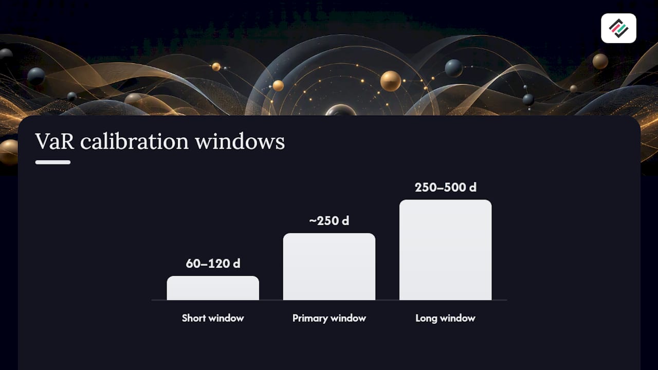
Window length is the first decision point. A short window (60 to 120 days) reacts fast to new volatility regimes but is noisy and can whipsaw your VaR number month to month. A long window (250 to 500 days) is stable but slow to reflect genuine structural shifts, like a currency moving from a managed peg to a float. Most desks split the difference: a primary window of roughly one year, supplemented by a shorter stress window for comparison.
Cleaning matters more than most modelers admit. FX data has real gaps around holidays across different jurisdictions, and a naive fill can introduce phantom zero-return days that quietly deflate your volatility estimate. Standard practice includes:
- Winsorizing extreme outliers rather than deleting them, to avoid discarding genuine crisis information.
- Aligning trading calendars across all currency pairs so a US holiday does not create a false flat day in a pair that trades actively in Asia.
- Choosing end-of-day snapshots consistently at the same cutoff time zone, since mixing London and New York closes introduces artificial jumps.
Correlation stability is the quiet risk in multi-currency books. Correlations between pairs can shift sharply during stress, sometimes reversing sign entirely, which breaks diversification assumptions baked into a variance-covariance model. Shrinkage techniques, blending the sample correlation matrix toward a more stable target, reduce estimation noise, particularly for illiquid pairs with thin history. The RBA's notes on covariance estimation recommend supplementing thin data with proxy or implied-volatility inputs, always documented and sensitivity-tested, rather than defaulting to generic market data.
Backtesting: Hit Rates, Exceptions, and Regulatory Expectations
Backtesting is not optional paperwork. It is the only real evidence that a VaR model works, and both the FCA and Basel frameworks expect it documented.
A 95% VaR model should see actual losses exceed the VaR threshold on roughly 1 trading day in 20, averaged over a full backtesting cycle. A 99% model should see exceptions closer to 1 in 100 days. If exceptions cluster (three breaches in a single volatile week rather than spread evenly) that pattern matters more than the raw count, since it signals the model is missing a volatility regime shift rather than just having bad luck.
Run the validation process in this order:
- Compare daily realized P&L against the prior day's VaR forecast over a rolling 250-day window.
- Count exceptions and compare against the expected frequency for your confidence level.
- Check for exception clustering using a statistical test, not just a visual scan.
- Document every parameter change with a dated rationale, since auditors expect a model-change log, not verbal history.
- Recalibrate volatility inputs or the underlying method if exceptions exceed the expected band for two consecutive quarters.
Expected exception frequency: for a 95% VaR model backtested over 250 trading days, roughly 12 to 13 exceptions is the statistically expected range, per FCA BIPRU7 guidance. Materially more than that, and the model is underestimating risk; materially fewer, and it may be overly conservative, tying up hedging budget unnecessarily.
Scenario analysis and stress testing supplement, rather than replace, statistical backtesting. Running the current portfolio through a historical stress episode, or a hypothetical shock like a sudden 15% devaluation, catches risks that a well-behaved 250-day backtest can miss entirely.
Turning VaR Into Treasury Limits and Hedging Decisions
A VaR number is only useful once it becomes a decision rule. That starts with matching the VaR horizon to the actual cash flow or hedge cycle, not the regulatory default. A corporate hedging a 90-day receivable should not lean on a 1-day VaR scaled up mechanically; it should use a horizon that reflects the real exposure window, a point CorpHedge's treasury guide covers in more operational detail.
From there, VaR feeds three kinds of limits:
- Position limits cap the notional size of an unhedged exposure to any single currency pair.
- Risk limits cap the VaR figure itself, often expressed as a percentage of EBITDA or free cash flow.
- Loss limits trigger a mandatory hedging or de-risking action once realized losses breach a threshold, independent of what the VaR model currently says.
Converting a VaR reading into hedge coverage is a judgment call layered on a number. A treasury team seeing VaR climb toward its risk limit has two levers: increase forward cover to lock in a known rate, or buy options to cap downside while keeping upside participation. Forwards are cheaper and simpler; options cost a premium but suit teams uncertain whether the exposure will materialize at all, like a bid still pending award. CorpHedge's guide to VaR-based hedging walks through how to size that coverage decision against a VaR reading.
Pro Tip: Set your risk limit at a level that leaves headroom for one bad backtesting quarter. A limit set right at your model's current VaR output gives you zero room to react before a breach forces an emergency hedge at a worse price.
Advanced Extensions: EVT, CAViaR, and Machine Learning Approaches
Standard VaR models handle normal market conditions well and crisis periods poorly. Extreme Value Theory (EVT) fits a distribution specifically to the tail of the return data rather than the whole sample, giving a materially better estimate of losses beyond the 99th percentile. It is worth the added complexity for any book with meaningful exposure to emerging-market or historically volatile pairs.
CAViaR (Conditional Autoregressive Value at Risk) models the VaR quantile directly as a time series rather than deriving it from a full distributional assumption, which can adapt faster to changing volatility regimes than standard parametric approaches.
For portfolios spanning many currency pairs, multivariate GARCH and principal component analysis (PCA) reduce the dimensionality problem: instead of estimating volatility and correlation for every pair individually, PCA identifies the handful of common factors driving most of the joint movement.
- EVT and CAViaR earn their complexity specifically for tail risk and crisis-period accuracy.
- Multivariate GARCH and PCA make sense once you are running VaR across eight or more currency pairs simultaneously.
- Machine learning and probabilistic forecasting can capture non-linear dynamics standard models miss, but overfitting risk is real and governance requirements, documentation, explainability, independent validation, do not disappear just because the model is more sophisticated. A note from the FCA and practitioner discussion on model limits underscores that VaR outputs, however generated, should never stand alone as the single risk number driving a decision.
How CorpHedge Supports the FX VaR Workflow
CorpHedge's platform tracks currency exposure in real time, applies VaR-based strategy logic, and connects with partner systems like Corpay for execution. Teams building out this capability internally can also work through the FX hedging course for a structured path through the concepts covered above.
FX VaR Compared to CVaR and Expected Shortfall
VaR answers one question: what is the maximum expected loss at a given confidence level over a given horizon? It does not say anything about how bad losses get beyond that threshold, which is exactly the gap Conditional VaR (CVaR), also called Expected Shortfall, fills.
Expected Shortfall calculates the average loss in the worst-case scenarios beyond the VaR cutoff, not just the cutoff itself. A 95% VaR of $2 million tells you losses should not exceed that figure 95% of the time.
For FX portfolios with meaningful optionality or exposure to historically volatile pairs, Expected Shortfall is arguably the more honest number, since it does not go blind exactly where risk matters most. It also has a mathematical property VaR lacks: subadditivity, meaning the Expected Shortfall of a combined portfolio can never exceed the sum of its parts, which makes it more reliable for aggregating risk across business units.
The practical answer is not choosing one over the other. Most sophisticated treasury and risk functions report both: VaR for its speed, familiarity, and ease of communication to a board, and Expected Shortfall as the tail-risk check that catches what VaR structurally cannot see. Basel's market risk framework has already shifted trading-book capital calculations toward Expected Shortfall for this exact reason, a signal that the rest of the risk management profession is likely to follow over time.
Liquidity, Market Microstructure, and What They Do to VaR
FX VaR models built on mid-price returns quietly assume you can exit a position at that mid-price whenever needed. That assumption fails precisely when it matters most: during a liquidity crunch, when bid-ask spreads on emerging-market or exotic pairs can widen sharply within minutes.
Market microstructure effects, spread widening, reduced quote depth, and gapping between quoted prices, mean that realized exit costs during stress routinely exceed what mid-price VaR predicts. A model calibrated entirely on liquid G10 pairs like EUR/USD or GBP/USD will systematically understate risk when applied to a book that also holds thinner pairs.
Two adjustments help close that gap. First, add a liquidity haircut or spread-cost buffer to VaR outputs for less liquid pairs, sized off historical spread behavior during past stress episodes rather than current calm-market spreads. Second, monitor quote depth and trading volume as a standalone risk signal alongside VaR itself, since a currency pair can show stable volatility right up until liquidity evaporates.
This matters more for corporates than it might first appear. A company hedging exposure in a frontier or emerging-market currency, common for firms with manufacturing or sales operations outside core G10 markets, needs to treat liquidity risk as a distinct line item, not something VaR alone will surface.
Implementation Challenges and the Software Layer
Building an FX VaR model is rarely the hard part. Sustaining it in production, with clean daily data feeds, a governance process, and outputs that actually reach the people making hedging decisions, is where most implementations stall.
The most common failure points are data pipeline gaps (a missed daily feed silently freezes the volatility estimate), model drift (nobody re-validates parameters after the analyst who built the model moves on), and a reporting gap between the risk team's output and the treasury desk's actual decision cadence. A VaR report that lands weekly is close to useless for a desk that adjusts hedge coverage daily.
Spreadsheet-based VaR models remain common at smaller corporates, largely because they are cheap to start. They also break down fast once the currency-pair count grows past a handful, since correlation matrices and historical windows become unwieldy to maintain by hand, and version control on a shared spreadsheet is a known source of silent errors. Purpose-built platforms that automate the data ingestion, calculation, and backtesting loop remove that maintenance burden and, more importantly, make the model-change log and validation history straightforward to produce when an auditor asks for it.
Regulatory Requirements and Compliance Considerations
FX VaR sits inside a broader market-risk regulatory framework, and the compliance bar depends on what kind of entity is running the model. Banks and regulated financial institutions face formal capital-adequacy requirements under Basel frameworks, with specific backtesting and validation obligations spelled out in the FCA's BIPRU7 handbook. Non-financial corporates hedging commercial FX exposure are not typically subject to the same capital rules, but auditors and lenders increasingly expect documented risk management processes, and a VaR model without a backtesting record and change log will draw scrutiny in any serious audit.
The core compliance expectations, regardless of entity type, are consistent: documented model assumptions, a defined backtesting schedule, a clear escalation path when exceptions exceed the expected frequency, and an independent review of the model separate from the team that built it. The FCA's guidance frames this as validation and remediation procedure, not a one-time approval. A model that passed review two years ago and has not been re-tested since is not compliant in any meaningful sense, even if nobody has formally flagged it.
For companies expanding into new currency exposure, entering Polish zloty or Swedish krona exposure through new operations, for instance, the compliance question is less about a specific regulatory threshold and more about whether the existing model, calibrated on established G10 pairs, actually extends cleanly to a less liquid or more locally-driven currency. That is a data and governance question first, and a regulatory one second.
Case Studies: VaR Under Different Market Conditions
Consider three distinct regimes and how the same variance-covariance model performs in each.
Calm, range-bound markets. In a period of low realized volatility, say EUR/USD trading in a tight band for several months, a standard parametric VaR model tracks realized losses closely. This is the environment where VaR earns the least skepticism and, not coincidentally, the environment where risk teams are most likely to get complacent about recalibration.
A sudden rate-driven shock. When a central bank surprises the market, a sharp repricing across a currency pair within a single session, a model calibrated on the preceding calm period will underestimate the loss almost every time. This is exactly the scenario where EWMA's faster reaction to new volatility outperforms a slower-moving GARCH baseline, and where a natural-horizon VaR built on a genuinely stressed historical window would have flagged the risk earlier than a model relying on trailing 12-month data alone.
A structural regime change. A currency moving from a managed or pegged regime to a free float is the hardest case for any model. Historical data from the pegged period is close to useless for volatility estimation once the float begins, since the entire statistical relationship the model was built on no longer holds. The only real defense here is qualitative: treat any regime-change currency as requiring a fresh model build with a shortened window and heavy reliance on comparable-currency proxies until enough new data accumulates.
The Governance-First View on FX VaR
The gap between a model that looks sound on a slide and one that actually protects a treasury function is governance, not sophistication. A VaR number nobody challenges quarterly, backtests rigorously, or stress-tests against a real scenario is decoration, not risk management. The teams that get this right treat every VaR figure as a hypothesis to be re-tested, not a fact to be reported.
— Bartas
CorpHedge: Turning FX VaR Into a Daily Workflow
Building the model is one project. Running it every day, backtesting it every quarter, and getting the number in front of the right person before a hedge decision is due, that is the part most in-house teams underestimate. CorpHedge's platform automates the exposure tracking, VaR calculation, and alerting loop described throughout this guide, so your risk figure is live instead of a monthly spreadsheet exercise.

The platform's VaR-based hedging feature applies the same variance-covariance and historical simulation logic covered above directly to your live currency positions, with integrations to execution partners like Corpay built in. Corporates hedging zloty or krona exposure can benefit from real-time tracking and VaR discipline similar to that used for G10 books. For teams that want to build internal capability rather than fully outsource it, the FX hedging course is a paid program covering practical hedging decisions. Start with a look at the platform's use cases to see where your current process has gaps.
Sources
- FCA handbook — BIPRU7 backtesting guidance
- IMF working paper 06/255 — Exchange rate risk measurement and management
- RBA research discussion paper RDP 9708 — Measuring traded market risk: VaR and backtesting techniques
This article is general information, not a substitute for advice from a qualified financial advisor. Consult a qualified financial professional about your own circumstances before acting on anything here.
FAQ
What Is a VaR Model?
In FX risk management, it converts currency exposure and volatility data into a single dollar or currency figure that tells a treasury team how much they could plausibly lose before action is warranted.
What Does a 95% VaR Mean?
Under proper backtesting per FCA guidance, that translates to roughly 1 exception day in every 20 over a full validation cycle.
What Are the Three Types of VaR?
The three primary FX VaR methods are variance-covariance (parametric), historical simulation, and Monte Carlo simulation. Parametric VaR is fastest but assumes normal returns, historical simulation captures real fat-tail behavior from past data, and Monte Carlo handles options and other non-linear positions that the other two methods struggle with.
How Do You Calculate Historical VaR?
Historical VaR reprices the current portfolio using actual historical daily returns, typically over a 250 to 500 day window, then ranks the resulting simulated profit-and-loss outcomes from worst to best.
Does CorpHedge Support FX VaR Calculations?
Yes. CorpHedge's platform applies VaR-based strategy logic directly to live currency exposure data, tracking positions and running the calculations described throughout this guide. Full platform details are available on the use cases page, and current pricing is listed on the CorpHedge site.